Funneling in Multilevel models

The first example

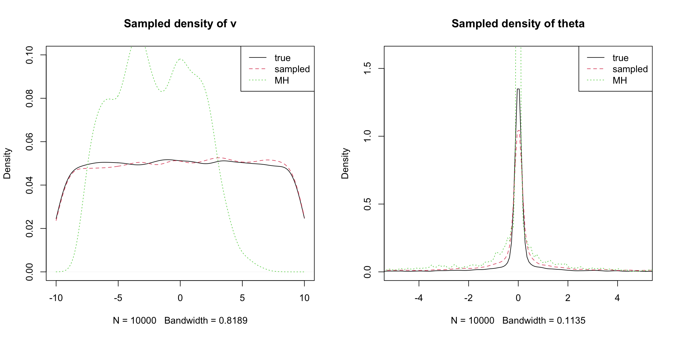
In the first example, we have the following model: \[ v\sim U(-10, 10),\\ \theta\sim N(0,\exp(2v)) \]

## simulate data
set.seed(1234)
NN <- 10000
A <- 10
v <- runif(NN, -A,A)
tau <- exp(v)
theta <- rnorm(NN) * tau

## Gibbs + MH sampling
MH_samples0 <- my_MH_sample0(10000, step_sizes = c(0.5, 0.5))

## JAGS sampling (Gibbs + slice)
library(runjags)
mod.jags <- "
model{
  theta ~ dnorm(0, exp(-v))
  v ~ dunif(-10,10)
}
"
jags.fit1 <- run.jags(mod.jags, n.chains = 1, sample = 10000, thin = 1,
                      burnin = 1000, adapt = 500, data = data.frame(x=1),
                      method = "parallel", modules = 'glm',
                      monitor=c("theta","v"))
samples <- as.matrix(jags.fit1$mcmc[[1]])
par(mfrow = c(1,3))
plot(theta, v, xlim=c(-20,20), ylim = c(-A,A), pch=20, cex=0.2,main="true")
plot(samples, xlim = c(-20,20),ylim = c(-A,A), pch=20, cex=0.2,main="JAGS")
plot(MH_samples0$theta, MH_samples0$v, xlim = c(-20,20),
     ylim = c(-10,10), pch=20, cex=0.2,main="my_MH")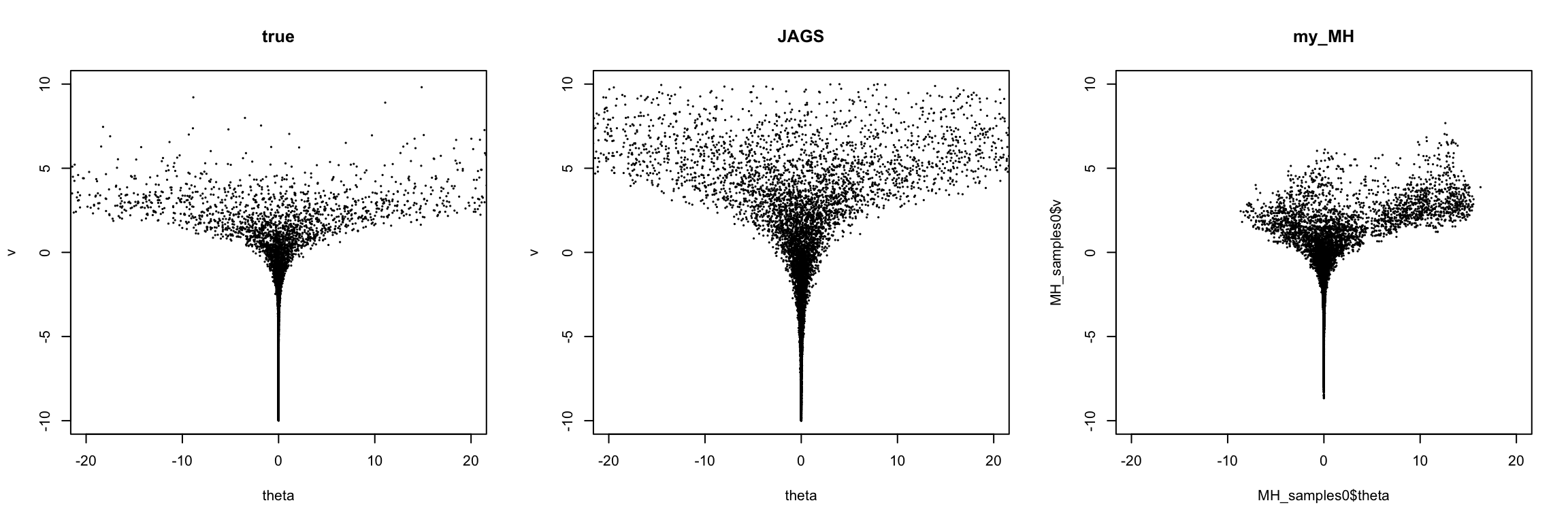

It can be seen that Gibbs + MH performs not well.

The second example

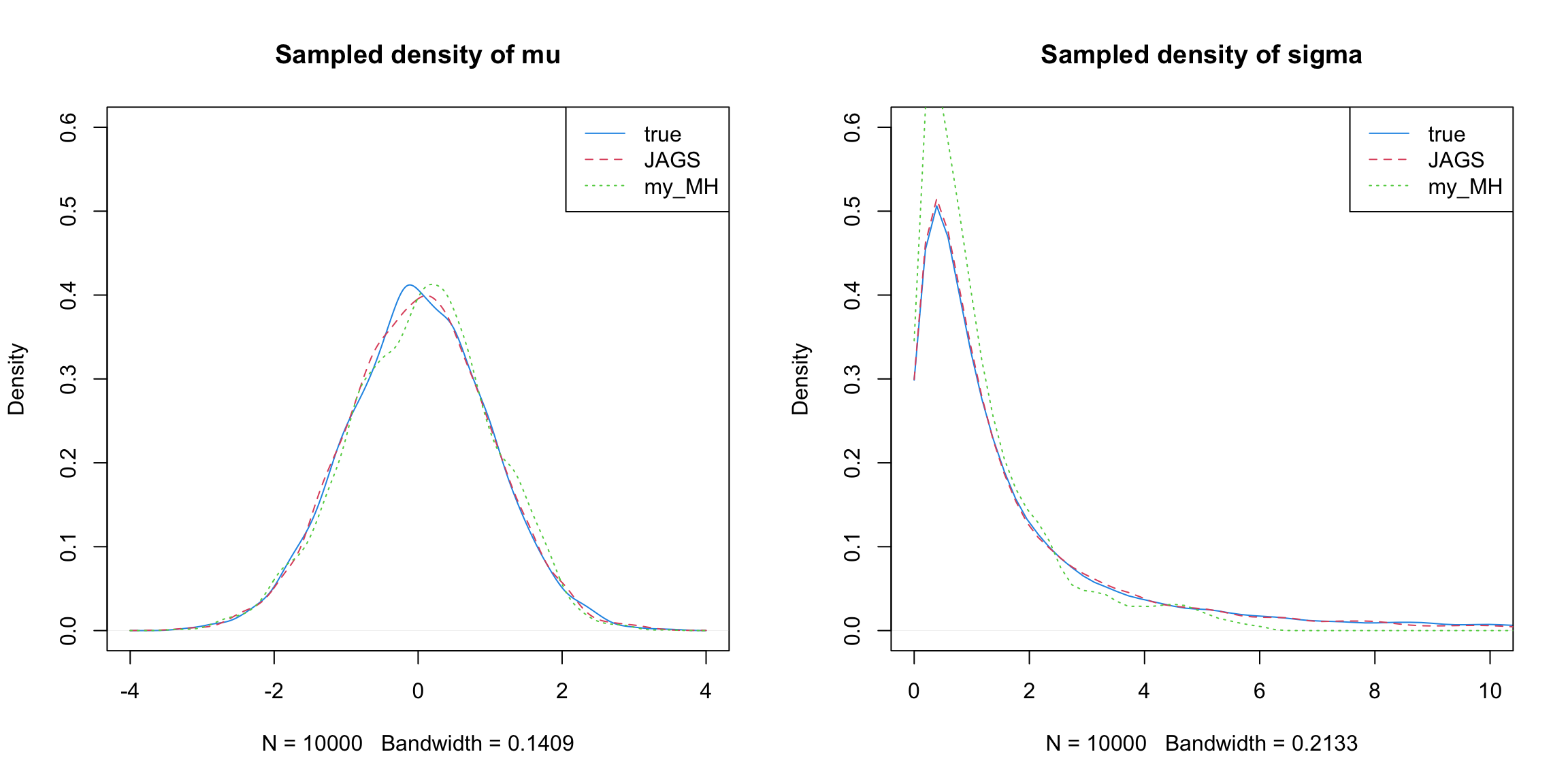
In the second simulation, we sample the following model: \[ y\sim N(\mu,\sigma^2),\\ \mu\sim N(0,1),\\ \sigma\sim\text{HalfCauchy}(1). \]

library(runjags)
set.seed(1234)
## Sample directly
NN <- 10000
mu = rnorm(NN)
sigma = abs(rcauchy(NN))
y <- mu + rnorm(NN) * sigma

## sample using JAGS
mod.jags <- "
model{
  y ~ dnorm(mu, tau)
  mu ~ dnorm(0, 1)
  sigma ~ dt(0, 1, 1)T(0,)
  tau = 1/sigma
}
"
jags.fit1 <- run.jags(mod.jags, n.chains = 1, sample = 10000, thin = 1,
                      burnin = 1000, adapt = 500, data = data.frame(x=1),
                      method = "parallel", modules = 'glm',
                      monitor=c("sigma", "mu", "y"))
samples <- as.matrix(jags.fit1$mcmc[[1]])

## sample using my MH sampler
MH_samples <- my_MH_sampler(10000, step_sizes = c(1, 0.2, 1))

## plot
par(mfrow=c(3,2))
plot(y, mu, xlim = c(-5,5),ylim=c(-4,4),pch=20, cex=0.2, main = "true")
plot(y, sigma, xlim = c(-5,5),ylim=c(0,2.5), pch=20, cex=0.2)
plot(samples[,c(3,2)], xlim = c(-5,5),ylim=c(-4,4), cex=0.2,pch=20, main = "JAGS")
plot(samples[,c(3,1)], xlim = c(-5,5),ylim=c(0,2.5),pch=20, cex=0.2)
plot(MH_samples$y, MH_samples$mu,xlim = c(-5,5),ylim=c(-4,4), pch=20, cex=0.2, main = "my_MH")
plot(MH_samples$y, MH_samples$sigma,xlim = c(-5,5),ylim=c(0,2.5), pch=20, cex=0.2)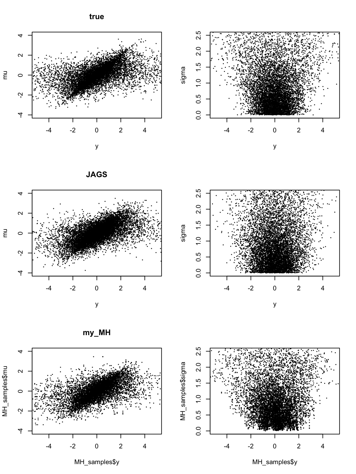

Conclusions

We observe for the above two simple case, only vanilla Gibbs+MH sampler suffers. Gibbs+Slice sampler performs well.

References

• Hierarchical Modeling by Michael Betancourt
• Funneling
• Betancourt and Girolami (2015)